
Linear Regression
A linear regression is constructed by fitting a line through a scatter plot of paired observations between two variables. The sketch below illustrates an example of a linear regression line drawn through a series of (X, Y) observations:
Figure 2.16: Linear Regression
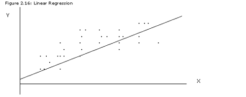 |
A linear regression line is usually determined quantitatively by a best-fit procedure such as least squares (i.e. the distance between the regression line and every observation is minimized). In linear regression, one variable is plotted on the X axis and the other on the Y. The X variable is said to be the independent variable, and the Y is said to be the dependent variable. When analyzing two random variables, you must choose which variable is independent and which is dependent. The choice of independent and dependent follows from the hypothesis - for many examples, this distinction should be intuitive. The most popular use of regression analysis is on investment returns, where the market index is independent while the individual security or mutual fund is dependent on the market. In essence, regression analysis formulates a hypothesis that the movement in one variable (Y) depends on the movement in the other (X).
Regression Equation
The regression equation describes the relationship between two variables and is given by the general format:
|
Where: Y = dependent variable; X = independent variable, a = intercept of regression line; b = slope of regression line, ε = error term
In this format, given that Y is dependent on X, the slope b indicates the unit changes in Y for every unit change in X. If b = 0.66, it means that every time X increases (or decreases) by a certain amount, Y increases (or decreases) by 0.66*that amount. The intercept a indicates the value of Y at the point where X = 0. Thus if X indicated market returns, the intercept would show how the dependent variable performs when the market has a flat quarter where returns are 0. In investment parlance, a manager has a positive alpha because a linear regression between the manager's performance and the performance of the market has an intercept number a greater than 0.
Linear Regression - Assumptions
Drawing conclusions about the dependent variable requires that we make six assumptions, the classic assumptions in relation to the linear regression model:
- The relationship between the dependent variable Y and the independent variable X is linear in the slope and intercept parameters a and b. This requirement means that neither regression parameter can be multiplied or divided by another regression parameter (e.g. a/b), and that both parameters are raised to the first power only. In other words, we can't construct a linear model where the equation was Y = a + b2X + ε, as unit changes in X would then have a b2 effect on a, and the relation would be nonlinear.
- The independent variable X is not random.
- The expected value of the error term "ε" is 0. Assumptions #2 and #3 allow the linear regression model to produce estimates for slope b and intercept a.
- The variance of the error term is constant for all observations. Assumption #4 is known as the "homoskedasticity assumption". When a linear regression is heteroskedastic its error terms vary and the model may not be useful in predicting values of the dependent variable.
- The error term ε is uncorrelated across observations; in other words, the covariance between the error term of one observation and the error term of the other is assumed to be 0. This assumption is necessary to estimate the variances of the parameters.
- The distribution of the error terms is normal. Assumption #6 allows hypothesis-testing methods to be applied to linear-regression models.
Standard Error of Estimate
Abbreviated SEE, this measure gives an indication of how well a linear regression model is working. It compares actual values in the dependent variable Y to the predicted values that would have resulted had Y followed exactly from the linear regression. For example, take a case where a company's financial analyst has developed a regression model relating annual GDP growth to company sales growth by the equation Y = 1.4 + 0.8X.
Assume the following experience (on the next page) over a five-year period; predicted data is a function of the model and GDP, and "actual" data indicates what happened at the company:
Year | (Xi) GDP growth | Predicted co. growth (Yi) | Actual co. Growth (Yi) | Residual(Yi - Yi) | Squared residual |
1 | 5.1 | 5.5 | 5.2 | -0.3 | 0.09 |
2 | 2.1 | 3.1 | 2.7 | -0.4 | 0.16 |
3 | -0.9 | 0.7 | 1.5 | 0.8 | 0.64 |
4 | 0.2 | 1.6 | 3.1 | 1.5 | 2.25 |
5 | 6.4 | 6.5 | 6.3 | -0.2 | 0.04 |
To find the standard error of the estimate, we take the sum of all squared residual terms and divide by (n - 2), and then take the square root of the result. In this case, the sum of the squared residuals is 0.09+0.16+0.64+2.25+0.04 = 3.18. With five observations, n - 2 = 3, and SEE = (3.18/3)1/2 = 1.03%.
The computation for standard error is relatively similar to that of standard deviation for a sample (n - 2 is used instead of n - 1). It gives some indication of the predictive quality of a regression model, with lower SEE numbers indicating that more accurate predictions are possible. However, the standard-error measure doesn't indicate the extent to which the independent variable explains variations in the dependent model.
Coefficient of Determination
Like the standard error, this statistic gives an indication of how well a linear-regression model serves as an estimator of values for the dependent variable. It works by measuring the fraction of total variation in the dependent variable that can be explained by variation in the independent variable.
In this context, total variation is made up of two fractions:
Total variation = explained variation + unexplained variation
total variation total variation
The coefficient of determination, or explained variation as a percentage of total variation, is the first of these two terms. It is sometimes expressed as 1 - (unexplained variation / total variation).
For a simple linear regression with one independent variable, the simple method for computing the coefficient of determination is squaring the correlation coefficient between the dependent and independent variables. Since the correlation coefficient is given by r, the coefficient of determination is popularly known as "R2, or R-squared". For example, if the correlation coefficient is 0.76, the R-squared is (0.76)2 = 0.578. R-squared terms are usually expressed as percentages; thus 0.578 would be 57.8%. A second method of computing this number would be to find the total variation in the dependent variable Y as the sum of the squared deviations from the sample mean. Next, calculate the standard error of the estimate following the process outlined in the previous section. The coefficient of determination is then computed by (total variation in Y - unexplained variation in Y) / total variation in Y. This second method is necessary for multiple regressions, where there is more than one independent variable, but for our context we will be provided the r (correlation coefficient) to calculate an R-squared.
What R2 tells us is the changes in the dependent variable Y that are explained by changes in the independent variable X. R2 of 57.8 tells us that 57.8% of the changes in Y result from X; it also means that 1 - 57.8% or 42.2% of the changes in Y are unexplained by X and are the result of other factors. So the higher the R-squared, the better the predictive nature of the linear-regression model.
Regression Coefficients
For either regression coefficient (intercept a, or slope b), a confidence interval can be determined with the following information:
- An estimated parameter value from a sample
- Standard error of the estimate (SEE)
- Significance level for the t-distribution
- Degrees of freedom (which is sample size - 2)
For a slope coefficient, the formula for confidence interval is given by b ± tc*SEE, where tc is the critical t value at our chosen significant level.
To illustrate, take a linear regression with a mutual fund's returns as the dependent variable and the S&P 500 index as the independent variable. For five years of quarterly returns, the slope coefficient b is found to be 1.18, with a standard error of the estimate of 0.147. Student's t-distribution for 18 degrees of freedom (20 quarters - 2) at a 0.05 significance level is 2.101. This data gives us a confidence interval of 1.18 ± (0.147)*(2.101), or a range of 0.87 to 1.49. Our interpretation is that there is only a 5% chance that the slope of the population is either less than 0.87 or greater than 1.49 - we are 95% confident that this fund is at least 87% as volatile as the S&P 500, but no more than 149% as volatile, based on our five-year sample.
Hypothesis testing and Regression Coefficients
Regression coefficients are frequently tested using the hypothesis-testing procedure. Depending on what the analyst is intending to prove, we can test a slope coefficient to determine whether it explains chances in the dependent variable, and the extent to which it explains changes. Betas (slope coefficients) can be determined to be either above or below 1 (more volatile or less volatile than the market). Alphas (the intercept coefficient) can be tested on a regression between a mutual fund and the relevant market index to determine whether there is evidence of a sufficiently positive alpha (suggesting value added by the fund manager).
The mechanics of hypothesis testing are similar to the examples we have used previously. A null hypothesis is chosen based on a not-equal-to, greater-than or less-than-case, with the alternative satisfying all values not covered in the null case. Suppose in our previous example where we regressed a mutual fund's returns on the S&P 500 for 20 quarters our hypothesis is that this mutual fund is more volatile than the market. A fund equal in volatility to the market will have slope b of 1.0, so for this hypothesis test, we state the null hypothesis (H0)as the case where slope is less than or greater to 1.0 (i.e. H0: b < 1.0). The alternative hypothesis Ha has b > 1.0. We know that this is a greater-than case (i.e. one-tailed) - if we assume a 0.05 significance level, t is equal to 1.734 at degrees of freedom = n - 2 = 18.
Example: Interpreting a Hypothesis Test
From our sample, we had estimated b of 1.18 and standard error of 0.147. Our test statistic is computed with this formula: t = estimated coefficient - hypothesized coeff. / standard error = (1.18 - 1.0)/0.147 = 0.18/0.147, or t = 1.224.
For this example, our calculated test statistic is below the rejection level of 1.734, so we are not able to reject the null hypothesis that the fund is more volatile than the market.
Interpretation: the hypothesis that b > 1 for this fund probably needs more observations (degrees of freedom) to be proven with statistical significance. Also, with 1.18 only slightly above 1.0, it is quite possible that this fund is actually not as volatile as the market, and we were correct to not reject the null hypothesis.
Example: Interpreting a regression coefficient.
The CFA exam is likely to give the summary statistics of a linear regression and ask for interpretation. To illustrate, assume the following statistics for a regression between a small-cap growth fund and the Russell 2000 index:
| Correlation coefficient | 0.864 |
| Intercept | -0.417 |
| Slope | 1.317 |
What do each of these numbers tell us?
- Variation in the fund is about 75%, explained by changes in the Russell 2000 index. This is true because the square of the correlation coefficient, (0.864)2 = 0.746, gives us the coefficient of determination or R-squared.
- The fund will slightly underperform the index when index returns are flat. This results from the value of the intercept being -0.417. When X = 0 in the regression equation, the dependent variable is equal to the intercept.
- The fund will on average be more volatile than the index. This fact follows from the slope of the regression line of 1.317 (i.e. for every 1% change in the index, we expect the fund's return to change by 1.317%).
- The fund will outperform in strong market periods, and underperform in weak markets. This fact follows from the regression. Additional risk is compensated with additional reward, with the reverse being true in down markets. Predicted values of the fund's return, given a return for the market, can be found by solving for Y = -0.417 + 1.317X (X = Russell 2000 return).
Analysis of Variance (ANOVA)
Analysis of variance, or ANOVA, is a procedure in which the total variability of a random variable is subdivided into components so that it can be better understood, or attributed to each of the various sources that cause the number to vary.
Applied to regression parameters, ANOVA techniques are used to determine the usefulness in a regression model, and the degree to which changes in an independent variable X can be used to explain changes in a dependent variable Y. For example, we can conduct a hypothesis-testing procedure to determine whether slope coefficients are equal to zero (i.e. the variables are unrelated), or if there is statistical meaning to the relationship (i.e. the slope b is different from zero). An F-test can be used for this process.
F-Test
The formula for F-statistic in a regression with one independent variable is given by the following:
|
The two abbreviations to understand are RSS and SSE:
- RSS, or the regression sum of squares, is the amount of total variation in the dependent variable Y that is explained in the regression equation. The RSS is calculated by computing each deviation between a predicted Y value and the mean Y value, squaring the deviation and adding up all terms. If an independent variable explains none of the variations in a dependent variable, then the predicted values of Y are equal to the average value, and RSS = 0.
- SSE, or the sum of squared error of residuals, is calculated by finding the deviation between a predicted Y and an actual Y, squaring the result and adding up all terms.
TSS, or total variation, is the sum of RSS and SSE. In other words, this ANOVA process breaks variance into two parts: one that is explained by the model and one that is not. Essentially, for a regression equation to have high predictive quality, we need to see a high RSS and a low SSE, which will make the ratio (RSS/1)/[SSE/(n - 2)] high and (based on a comparison with a critical F-value) statistically meaningful. The critical value is taken from the F-distribution and is based on degrees of freedom.
For example, with 20 observations, degrees of freedom would be n - 2, or 18, resulting in a critical value (from the table) of 2.19. If RSS were 2.5 and SSE were 1.8, then the computed test statistic would be F = (2.5/(1.8/18) = 25, which is above the critical value, which indicates that the regression equation has predictive quality (b is different from 0)
Estimating Economic Statistics with Regression Models
Regression models are frequently used to estimate economic statistics such as inflation and GDP growth. Assume the following regression is made between estimated annual inflation (X, or independent variable) and the actual number (Y, or dependent variable):
Y = 0.154 + 0.917X
Using this model, the predicted inflation number would be calculated based on the model for the following inflation scenarios:
Inflation estimate | Inflation based on model |
-1.1% | -0.85% |
+1.4% | +1.43% |
+4.7% | +4.46% |
The predictions based on this model seem to work best for typical inflation estimates, and suggest that extreme estimates tend to overstate inflation - e.g. an actual inflation of just 4.46 when the estimate was 4.7. The model does seem to suggest that estimates are highly predictive. Though to better evaluate this model, we would need to see the standard error and the number of observations on which it is based. If we know the true value of the regression parameters (slope and intercept), the variance of any predicted Y value would be equal to the square of the standard error.
In practice, we must estimate the regression parameters; thus our predicted value for Y is an estimate based on an estimated model. How confident can we be in such a process? In order to determine a prediction interval, employ the following steps:
1. Predict the value of the dependent variable Y based on independent observation X.
2. Compute the variance of the prediction error, using the following equation:
Formula 2.42 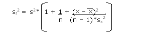 |
Where: s2 is the squared standard error of the estimate, n is number of observations, X is the value of the independent variable used to make the prediction, X is the estimated mean value of the independent variable, and sx2 is the variance of X.
3. Choose a significance level α for the confidence interval.
4. Construct an interval at (1 - α) percent confidence, using the structure Y ± tc*sf.
Here's another case where the material becomes much more technical than necessary and one can get bogged down in preparing, when in reality the formula for variance of a prediction error isn't likely to be covered. Prioritize - don't squander precious study hours memorizing it. If the concept is tested at all, you'll likely be given the answer to Part 2. Simply know how to use the structure in Part 4 to answer a question.
For example, if the predicted X observation is 2 for the regression Y = 1.5 + 2.5X, we would have a predicted Y of 1.5 + 2.5*(2), or 6.5. Our confidence interval is 6.5 ± tc*sf. The t-stat is based on a chosen confidence interval and degrees of freedom, while sf is the square root of the equation above (for variance of the prediction error. If these numbers are tc = 2.10 for 95% confidence, and sf = 0.443, the interval is 6.5 ± (2.1)*(0.443), or 5.57 to 7.43.
Limitations of Regression Analysis
Focus on three main limitations:
1. Parameter Instability - This is the tendency for relationships between variables to change over time due to changes in the economy or the markets, among other uncertainties. If a mutual fund produced a return history in a market where technology was a leadership sector, the model may not work when foreign and small-cap markets are leaders.
2. Public Dissemination of the Relationship - In an efficient market, this can limit the effectiveness of that relationship in future periods. For example, the discovery that low price-to-book value stocks outperform high price-to-book value means that these stocks can be bid higher, and value-based investment approaches will not retain the same relationship as in the past.
3. Violation of Regression Relationships - Earlier we summarized the six classic assumptions of a linear regression. In the real world these assumptions are often unrealistic - e.g. assuming the independent variable X is not random.


0 comments:
Post a Comment