Common Probability Distribution Properties

CFA Level 1 - Quantitative Methods

Normal Distribution

The normal distribution is a continuous probability distribution that, when graphed as a probability density, takes the form of the so-called bell-shaped curve. The bell shape results from the fact that, while the range of possible outcomes is infinite (negative infinity to positive infinity), most of the potential outcomes tend to be clustered relatively close to the distribution's mean value. Just how close they are clustered is given by the standard deviation. In other words, a normal distribution is described completely by two parameters: its mean (μ) and its standard deviation (σ).

Here are other defining characteristics of the normal distribution: it is symmetric, meaning the mean value divides the distribution in half and one side is the exact mirror image of the other -that is, skewness = 0. Symmetry also requires that mean = median = mode. Its kurtosis (measure of peakedness) is 3 and its excess kurtosis (kurtosis - 3) equals 0. Also, if given 2 or more normally distributed random variables, the linear combination must also be normally distributed.

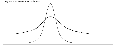
While any normal distribution will share these defining characteristics, the mean and standard deviation will be unique to the random variable, and these differences will affect the shape of the distribution. On the following page are two normal distributions, each with the same mean, but the distribution with the dotted line has a higher standard deviation.




Univariate vs. Multivariate Distributions

A univariate distribution specifies probabilities for a single random variable, while a multivariate distribution combines the outcomes of a group of random variables and summarizes probabilities for the group. For example, a stock will have a distribution of possible return outcomes; those outcomes when summarized would be in a univariable distribution. A portfolio of 20 stocks could have return outcomes described in terms of 20 separate univariate distributions, or as one multivariate distribution.

Earlier we indicated that a normal distribution is completely described by two parameters: its mean and standard deviation. This statement is true of a univariate distribution. For models of multivariate returns, the mean and standard deviation of each variable do not completely describe the multivariate set. A third parameter is required, the correlation, or co-movement, between each pair of variables in the set. For example, if a multivariate return distribution was being assembled for a portfolio of stocks, and a number of pairs were found to be inversely related (i.e. one increases at the same time the other decreases), then we must consider the overall effect on portfolio variance. For a group of assets that are not completely positively related, there is the opportunity to reduce overall risk (variance) as a result of the interrelationships.

For a portfolio distribution with n stocks, the multivariate distribution is completely described by the n mean returns, the n standard deviations and the n*(n - 1)/2 correlations. For a 20-stock portfolio, that's 20 lists of returns, 20 lists of variances of return and 20*19/2, or 190 correlations.

(See more) Confidence Intervals

| | Print This! | No comments

Do you like this post?